<?xml version="1.0" encoding="utf-8"?><feed xmlns="http://www.w3.org/2005/Atom" ><generator uri="https://jekyllrb.com/" version="3.10.0">Jekyll</generator><link href="https://yashsawant22.github.io/feed.xml" rel="self" type="application/atom+xml" /><link href="https://yashsawant22.github.io/" rel="alternate" type="text/html" /><updated>2026-05-09T20:21:27+00:00</updated><id>https://yashsawant22.github.io/feed.xml</id><title type="html">yash sawant</title><subtitle>writing about what I learn — training internals, post-training, building things from scratch</subtitle><author><name>Yash Sawant</name></author><entry><title type="html">Adaptive LoRA Rank Allocation Works for SFT. It Fails Under GRPO. Here’s Why.</title><link href="https://yashsawant22.github.io/2026/05/09/adaptive-lora-sft-vs-grpo.html" rel="alternate" type="text/html" title="Adaptive LoRA Rank Allocation Works for SFT. It Fails Under GRPO. Here’s Why." /><published>2026-05-09T00:00:00+00:00</published><updated>2026-05-09T00:00:00+00:00</updated><id>https://yashsawant22.github.io/2026/05/09/adaptive-lora-sft-vs-grpo</id><content type="html" xml:base="https://yashsawant22.github.io/2026/05/09/adaptive-lora-sft-vs-grpo.html"><![CDATA[<p>If you’ve fine-tuned a large language model in the last two years, you’ve probably used LoRA. The trick is so good and so cheap that it feels like a cheat code: instead of updating the model’s billions of parameters, you train a tiny pair of low-rank matrices alongside each weight matrix you care about. The model behaves as if you’d fine-tuned the whole thing, but you’ve touched maybe one or two percent of the parameter count.</p>

<p>The natural follow-up question, once you’ve used LoRA enough, is: <em>why do all layers get the same rank?</em></p>

<p>Empirically, transformer layers don’t contribute equally to whatever you’re fine-tuning on. Some are doing heavy lifting; some are barely moving. So if you have a fixed parameter budget, why not concentrate it where it matters?</p>

<p>This question kicked off an entire subfield of “adaptive rank allocation” methods over the past two years — and the punchline of every paper has been the same. Profile the gradients, allocate rank where the gradients are largest, save parameters, get the same accuracy. AdaLoRA. GoRA. IGU-LoRA. ILA. Aletheia. Five different angles on the same recipe, all under supervised fine-tuning, all reporting the same kind of win.</p>

<p>So I tried the recipe under GRPO — the RL algorithm DeepSeek popularized for training reasoning models.</p>

<p>It didn’t transfer. Adaptive allocation made the model <strong>worse</strong> than uniform.</p>

<p>This post is about why. The short version is that the gradient structure of GRPO is qualitatively different from SFT — flatter, more spread out, and more entangled with rank itself — and a recipe that depends on a peaked, sparse importance map quietly stops working when the importance map isn’t peaked or sparse anymore. The longer version has a surprise in it that has uncomfortable implications for the entire profile-then-reallocate paradigm.</p>

<hr />

<h2 id="the-adaptive-rank-story-under-sft">The adaptive-rank story under SFT</h2>

<p>Quick recap of the supervised case, because the rest of this post hinges on the contrast.</p>

<p>The original LoRA paper (<a href="https://arxiv.org/abs/2106.09685">Hu et al., 2022</a>) set rank uniformly across layers. Every adapter got, say, rank 8 or 16, regardless of what layer it was attached to. This was a reasonable default — you’re already saving 99% of parameters, so optimizing the last bit isn’t a priority.</p>

<p><strong>AdaLoRA</strong> (Zhang et al., 2023) was the first major paper to push back on this. The argument: not all weight updates matter equally during fine-tuning, so under a fixed parameter budget, you should pour rank into the high-importance directions and prune it away from the low-importance ones. AdaLoRA does this dynamically during training, parameterizing the LoRA decomposition as an SVD and pruning the small singular values as it learns which ones matter.</p>

<p>The key empirical finding behind AdaLoRA, and behind everything that followed, is that the importance distribution is <em>peaked</em>. Some layers and modules carry a lot of signal; others carry almost none. If you visualize the per-layer gradient magnitude during SFT, you see hot spots — usually concentrated in middle-to-late attention layers — and cold zones where the gradient is essentially noise.</p>

<p><strong>ILA</strong> (Shi et al., 2024) made this concrete in a clean way: under SFT, roughly <strong>30% of layers carry over 80% of the gradient signal</strong>. The rest are essentially passengers. Reduce their rank, redistribute that capacity into the hot layers, and you get the same downstream accuracy with a smaller parameter count. This is the free lunch that adaptive rank allocation has been compounding for two years.</p>

<p><strong>GoRA</strong> (He et al., 2025) extended the idea to dynamic during-training profiling rather than static profiling. <strong>IGU-LoRA</strong> (Cui et al., 2026) added a per-layer initialization variance correction so that adapters with different ranks start with comparable activation magnitudes. <strong>Aletheia</strong> (Saket, 2026) brought in a more rigorous information-theoretic objective on top of the same skeleton.</p>

<p>Different angles on the same recipe. Distilled, the recipe is:</p>

<ol>
  <li>Profile the per-layer gradient magnitude during a uniform-rank run.</li>
  <li>Allocate rank proportional to gradient importance, under a fixed total budget.</li>
  <li>Train.</li>
  <li>Win on the parameter-accuracy frontier.</li>
</ol>

<p>This works because the gradient signal under SFT is sparse. Take that sparsity away and the recipe loses its purchase.</p>

<hr />

<h2 id="what-changes-under-rl">What changes under RL</h2>

<p>GRPO — Group Relative Policy Optimization, from the <a href="https://arxiv.org/abs/2402.03300">DeepSeekMath paper</a> — looks superficially like another fine-tuning algorithm. You take a base model, compute per-token gradients, update the weights. The gradient just comes from a different objective: instead of cross-entropy against ground truth, you compute a reward over generated completions and shape the gradient using group-relative advantages.</p>

<p>So the natural question is: does the SFT recipe transfer? Profile the gradients during a GRPO run, redistribute rank where the gradients are large, train, save parameters?</p>

<p>The setup of the experiment was deliberately boring. Qwen 2.5 1.5B Instruct. GSM8K. GRPO with two rewards (format compliance and correctness). LoRA on all seven projection modules per layer (q/k/v/o/up/down/gate) — 28 layers × 7 modules = 196 adapters in total. Total rank budget held fixed at 896 across configurations (= 28 × 32, the uniform baseline) so every configuration had the same parameter count. The only thing varying was <em>where</em> that parameter mass was concentrated.</p>

<p>The strategies tested:</p>

<ul>
  <li><strong>Uniform</strong> — every layer rank 32. Baseline.</li>
  <li><strong>Proportional</strong> — gradient-aware. Hot layers get more rank, cold layers get less. Same total budget.</li>
  <li><strong>Reduced 70%</strong> — gradient-aware at 70% of the parameters. (How much budget can the recipe save?)</li>
  <li><strong>Random</strong> — same total budget, allocation drawn at random. Control.</li>
</ul>

<p>I expected the standard SFT result: proportional ≥ uniform &gt; random. What I got was:</p>

<table>
  <thead>
    <tr>
      <th>Strategy</th>
      <th>Rank Range</th>
      <th>Params</th>
      <th>GSM8K Acc</th>
    </tr>
  </thead>
  <tbody>
    <tr>
      <td>Base model (no LoRA)</td>
      <td>—</td>
      <td>0</td>
      <td>66.0%</td>
    </tr>
    <tr>
      <td>Reduced 70%</td>
      <td>r=12–31</td>
      <td>25.8M</td>
      <td>65.0%</td>
    </tr>
    <tr>
      <td>Random</td>
      <td>r=16–48</td>
      <td>36.9M</td>
      <td>67.5%</td>
    </tr>
    <tr>
      <td>Proportional (gradient-aware)</td>
      <td>r=20–40</td>
      <td>36.9M</td>
      <td>70.0%</td>
    </tr>
    <tr>
      <td><strong>Uniform (r=32)</strong></td>
      <td>r=32–32</td>
      <td><strong>36.9M</strong></td>
      <td><strong>74.5%</strong></td>
    </tr>
  </tbody>
</table>

<p>Uniform won. By 4.5 points over the gradient-aware proportional allocation that “should” have been the optimum.</p>

<p>The interesting twist: gradient-aware <em>did</em> beat random by 2.5 points. The gradient signal was real — proportional knew which layers were hotter than random did. It just wasn’t enough to overcome the cost of redistributing rank.</p>

<hr />

<h2 id="why-grpo-has-a-flatter-gradient-landscape">Why: GRPO has a flatter gradient landscape</h2>

<p>The first thing that came out of profiling was that the gradient distribution under GRPO looks nothing like the SFT story.</p>

<p><img src="/assets/img/grpo-heatmap.png" alt="Per-layer gradient magnitude across 1000 GRPO steps" /></p>

<p>
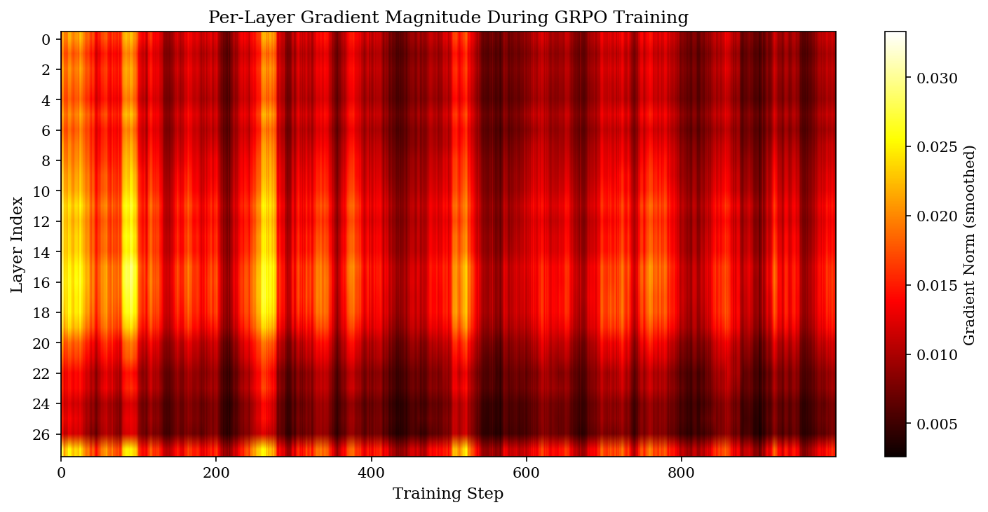
Under SFT (per ILA’s findings), the top 30% of layers carry over 80% of the gradient signal. Under GRPO in this run, the top 30% carry only <strong>~36%</strong>. The hottest layer (15) carries 4.68% of total gradient. The coldest (26) carries 2.15%. <strong>Max-to-min ratio: 2.17x.</strong></p>

<p>For comparison, SFT fine-tunes on similar architectures often show ratios of 10x or more. GRPO is essentially flat.</p>

<p>The flatness isn’t an artifact of averaging over noisy phases either. The early-vs-late training correlation of the importance map is <strong>0.962</strong> — it stabilizes within the first 100 steps and stays put. The structure is real, it’s just shallow.</p>

<p>This already gives you a clean story for the negative result. Adaptive rank allocation banks on the existence of idle layers whose capacity you can safely steal. Under SFT there are. Under GRPO there aren’t. Drop a layer’s rank from 32 to 20 and you’ve broken something the model needs.</p>

<p>But there was a second thing that came out of the profiling that I didn’t expect.</p>

<hr />

<h2 id="the-amplification-effect">The amplification effect</h2>

<p>I’d profiled gradients during <em>every</em> run, not just the uniform baseline, mostly to sanity-check that the rank allocation was applied correctly. When I plotted the gradient distribution for the proportional run alongside uniform:
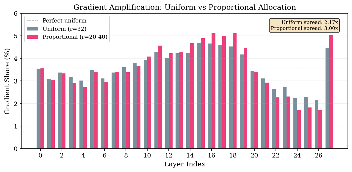
</p>

<p><img src="/assets/img/grpo-amplification.png" alt="Gradient amplification under non-uniform allocation" /></p>

<p>The spread <em>widens</em>. Uniform: 2.17x max/min. Proportional (same total budget): 3.00x. Reduced: 3.57x.</p>

<p>Hot layers given more rank absorbed <em>more</em> gradient. Cold layers given less rank went quieter. The allocation was creating a positive feedback loop — rank was concentrating gradient onto whichever layers had been given the rank.</p>

<p>That made me suspicious. Was the gradient just following itself? Was the proportional configuration simply amplifying its own profiling?</p>

<p>I ran the random allocation as a control. Layer 1 is normally one of the <em>coldest</em> layers — 3.09% of gradient under uniform. The random allocation gave it rank 48. Its gradient share jumped to <strong>4.21%</strong>, making it the second hottest layer in the network. Layer 15, normally the hottest, got rank 24 in the random allocation, and its gradient share dropped from 4.68% to 3.98%.</p>

<p>The correlation between allocated rank and gradient shift is <strong>0.972 for random, 0.946 for proportional.</strong></p>

<p>Read that line again. Even when rank is allocated <em>with no relation to gradient importance whatsoever</em>, the gradient follows. <strong>Rank determines gradient importance, not the other way around.</strong></p>

<p>This is the part of the result I didn’t expect, and it has uncomfortable implications for the entire profile-then-reallocate paradigm. The “important” layers your profiler identifies aren’t intrinsically important. They’re whatever layers happen to have rank to express themselves through. Move the rank, and the importance map moves with it.</p>

<p>This doesn’t necessarily falsify what the SFT papers found — under SFT, the importance map appears to be more anchored in the data and less in the rank distribution. But the moment you move to RL, where the gradient is shaped by sparse, noisy reward signals rather than dense supervision, the relationship inverts. Rank becomes a <em>cause</em> of importance, not a <em>consequence</em>.</p>

<hr />

<h2 id="a-practical-aside-pefts-silent-wildcard">A practical aside: PEFT’s silent wildcard</h2>

<p>Halfway through this work, my proportional run had 34.6M params instead of the expected 36.9M and no errors were thrown. Worth flagging because if you’re doing non-uniform LoRA in PEFT, you will hit this.</p>

<p>I had set up <code class="language-plaintext highlighter-rouge">rank_pattern</code> like this:</p>

<div class="language-python highlighter-rouge"><div class="highlight"><pre class="highlight"><code><span class="n">rank_pattern</span> <span class="o">=</span> <span class="p">{</span>
    <span class="s">"model.layers.15.*.q_proj"</span><span class="p">:</span> <span class="mi">40</span><span class="p">,</span>
    <span class="p">...</span>
<span class="p">}</span>
</code></pre></div></div>

<p>PEFT’s <code class="language-plaintext highlighter-rouge">rank_pattern</code> does not treat <code class="language-plaintext highlighter-rouge">*</code> as a glob. It’s a regex match against the full module path, and <code class="language-plaintext highlighter-rouge">*</code> in regex means “zero or more of the previous character.” So <code class="language-plaintext highlighter-rouge">model.layers.15.*.q_proj</code> matched essentially nothing in the actual module tree, every match silently fell back to the default rank, and the only signal anything was wrong was a slightly-off parameter count.</p>

<p>Fix: use exact paths.</p>

<div class="language-python highlighter-rouge"><div class="highlight"><pre class="highlight"><code><span class="n">rank_pattern</span> <span class="o">=</span> <span class="p">{</span>
    <span class="s">"model.layers.15.self_attn.q_proj"</span><span class="p">:</span> <span class="mi">40</span><span class="p">,</span>
    <span class="s">"model.layers.15.mlp.up_proj"</span><span class="p">:</span> <span class="mi">40</span><span class="p">,</span>
    <span class="p">...</span>
<span class="p">}</span>
</code></pre></div></div>

<p>Verify trainable parameter count after applying the config.</p>

<hr />

<h2 id="what-id-take-from-this">What I’d take from this</h2>

<p>Don’t naively port SFT-era rank allocation to RL training. SFT and RL appear to have qualitatively different gradient structures — peaked under SFT, flat under GRPO — and the techniques that exploit one don’t transfer. This is true even when the algorithm “looks like” fine-tuning at the gradient-step level.</p>

<p>The amplification finding has a stronger implication: <strong>static profiling can’t be the answer for RL.</strong> Whatever you measure during a uniform-rank run will shift the moment you reallocate. If adaptive rank is going to work under RL — and it might — it probably has to be <em>dynamic</em>, adjusting continuously during training (the AdaLoRA way), rather than committing to a fixed allocation upfront based on a profiling run.</p>

<p>The good news is that under GRPO, uniform is fine. It’s also the cheapest thing to do. If you’re allocating effort across an LLM training stack, you can move rank-allocation work down the priority list for RL workloads and spend the cycles somewhere they’ll actually pay off.</p>

<p>Negative results don’t always make great paper material. But this one was clarifying for me about what “transfer” actually means between fine-tuning regimes — and about how much of what we think we know about which layers matter is downstream of capacity allocation rather than upstream of it.</p>

<hr />

<p>The full paper is on arXiv (cs.CL, awaiting announcement). Code: <a href="https://github.com/yashsawant22/adaptive-lora-rank-grpo">github.com/yashsawant22/adaptive-lora-rank-grpo</a>. Submitted to the <a href="https://grigoris.ece.wisc.edu/workshops/colorai-icml-2026/">CoLoRAI workshop at ICML 2026</a>.</p>]]></content><author><name>Yash Sawant</name></author><summary type="html"><![CDATA[If you’ve fine-tuned a large language model in the last two years, you’ve probably used LoRA. The trick is so good and so cheap that it feels like a cheat code: instead of updating the model’s billions of parameters, you train a tiny pair of low-rank matrices alongside each weight matrix you care about. The model behaves as if you’d fine-tuned the whole thing, but you’ve touched maybe one or two percent of the parameter count.]]></summary></entry><entry><title type="html">Personalizing LLMs for High-Stakes Decisions: Four Lessons</title><link href="https://yashsawant22.github.io/2026/05/09/personalization-high-stakes-decisions.html" rel="alternate" type="text/html" title="Personalizing LLMs for High-Stakes Decisions: Four Lessons" /><published>2026-05-09T00:00:00+00:00</published><updated>2026-05-09T00:00:00+00:00</updated><id>https://yashsawant22.github.io/2026/05/09/personalization-high-stakes-decisions</id><content type="html" xml:base="https://yashsawant22.github.io/2026/05/09/personalization-high-stakes-decisions.html"><![CDATA[<p>Most LLM personalization research assumes the easy case: writing style, tone, topical preferences. What happens when personalization has to survive real consequences — when “getting the user what they want” and “getting the user what they need” actively diverge?</p>

<p>I spent the last several months building a personalized investment assistant for my own portfolio as a research testbed. The goal wasn’t a product — it was to see which parts of the standard personalization stack (RAG over user history, preference modeling, instruction tuning) actually hold up when the downstream decision costs money and the user’s stated preferences contradict their behavior.</p>

<p>Four things broke in ways I didn’t expect. This post is about those four things, because I think they generalize to any domain where LLM personalization meets consequential decisions — healthcare, legal, career coaching, long-horizon planning.</p>

<hr />

<h2 id="background-a-thesis-centric-architecture">Background: A Thesis-Centric Architecture</h2>

<p>Before the lessons, a quick mental model of the system, because the design choice matters for what follows.</p>

<p>Most LLM-over-finance setups start with price data and retrieve relevant news or filings. I inverted it: the primary unit of memory is <em>the user’s stated reasoning for holding a position</em> — a structured “thesis” — and every downstream component (reports, alerts, evaluation) scores new evidence against that thesis, not against the market in the abstract.</p>

<div class="language-plaintext highlighter-rouge"><div class="highlight"><pre class="highlight"><code>DATA SOURCES
  Brokerage (Robinhood) · Market Data (yfinance)
  Earnings Calendar · Your Interactions (CLI/Web/Chat)
          │
          ▼
CORE ENGINE
  ┌─────────────┐  ┌─────────────┐  ┌─────────────┐
  │ Living      │  │ Conviction  │  │ Behavioral  │
  │ Thesis      │  │ Scoring     │  │ Memory      │
  │ Manager     │  │ Engine      │  │ Extractor   │
  │             │  │             │  │             │
  │ Per-holding │  │ CONFIRMED   │  │ preferences │
  │ hypotheses  │  │ UNCHANGED   │  │ beliefs     │
  │ with break  │  │ WEAKENED    │  │ patterns    │
  │ conditions  │  │ BROKEN      │  │ rules       │
  └──────┬──────┘  └──────┬──────┘  │ risk toler. │
         │               │         └──────┬──────┘
         └───────┬────────┴───────────────┘
                 ▼
ANALYSIS LAYER
  Drift Detection · Pattern Matching · Position Grading
          │
          ▼
OUTPUT LAYER
  Daily Reports · Alerts · AI Chat · Web Dashboard
</code></pre></div></div>

<p>A thesis is not free-form text. It’s a structured object with fields the LLM must evaluate against:</p>

<div class="language-python highlighter-rouge"><div class="highlight"><pre class="highlight"><code><span class="o">@</span><span class="n">dataclass</span>
<span class="k">class</span> <span class="nc">Thesis</span><span class="p">:</span>
    <span class="n">ticker</span><span class="p">:</span> <span class="nb">str</span>
    <span class="n">conviction_statement</span><span class="p">:</span> <span class="nb">str</span>       <span class="c1"># "AI infra capex is in a multi-year buildout"
</span>    <span class="n">validation_triggers</span><span class="p">:</span> <span class="nb">list</span><span class="p">[</span><span class="nb">str</span><span class="p">]</span>  <span class="c1"># signals that would strengthen the thesis
</span>    <span class="n">break_conditions</span><span class="p">:</span> <span class="nb">list</span><span class="p">[</span><span class="nb">str</span><span class="p">]</span>     <span class="c1"># signals that would falsify it
</span>    <span class="n">catalysts</span><span class="p">:</span> <span class="nb">list</span><span class="p">[</span><span class="nb">str</span><span class="p">]</span>            <span class="c1"># upcoming events that resolve uncertainty
</span>    <span class="n">time_horizon</span><span class="p">:</span> <span class="nb">str</span>               <span class="c1"># "6-18 months"
</span>    <span class="n">conviction_score</span><span class="p">:</span> <span class="nb">float</span>         <span class="c1"># 0-10, updated over time
</span></code></pre></div></div>

<p>When new evidence arrives (an earnings print, a macro data point, a news headline), the scoring prompt forces the model to map the evidence onto <code class="language-plaintext highlighter-rouge">validation_triggers</code> and <code class="language-plaintext highlighter-rouge">break_conditions</code> explicitly — not to produce a free-form “bullish / bearish” verdict. The structured format is what makes the four problems below tractable at all.</p>

<hr />

<h2 id="four-things-that-broke">Four Things That Broke</h2>

<h3 id="1-the-users-profile-contradicts-itself--and-the-contradiction-is-the-signal">1. The user’s “profile” contradicts itself — and the contradiction is the signal</h3>

<p>Most personalization systems model the user as a stable preference vector. You extract preferences from history, you RAG over them, you condition generation on them. Done.</p>

<p>In a high-stakes domain, the user’s stated rules and their behavior routinely disagree — and flattening that disagreement into a single “preference” throws away the most useful signal in the data.</p>

<p>Concretely: I have a stated rule of “never average down into a position whose thesis is weakening.” My trade history shows I do exactly that during high-volatility stretches. A naive preference model either encodes the rule (and gives advice I’ll ignore) or encodes the behavior (and endorses the mistake). Neither is useful.</p>

<p>The fix was to stop collapsing these into one profile. Behavioral memory is split into five typed stores with different decay rates:</p>

<div class="language-python highlighter-rouge"><div class="highlight"><pre class="highlight"><code><span class="n">MEMORY_TYPES</span> <span class="o">=</span> <span class="p">{</span>
    <span class="s">"preference"</span><span class="p">:</span>    <span class="p">{</span><span class="s">"decay_days"</span><span class="p">:</span> <span class="mi">180</span><span class="p">},</span>  <span class="c1"># "prefers dividend payers"
</span>    <span class="s">"belief"</span><span class="p">:</span>        <span class="p">{</span><span class="s">"decay_days"</span><span class="p">:</span> <span class="mi">30</span><span class="p">},</span>   <span class="c1"># "thinks rates will cut in Q3"
</span>    <span class="s">"pattern"</span><span class="p">:</span>       <span class="p">{</span><span class="s">"decay_days"</span><span class="p">:</span> <span class="mi">90</span><span class="p">},</span>   <span class="c1"># "buys dips during VIX spikes"
</span>    <span class="s">"rule"</span><span class="p">:</span>          <span class="p">{</span><span class="s">"decay_days"</span><span class="p">:</span> <span class="mi">365</span><span class="p">},</span>  <span class="c1"># "never averages into broken theses"
</span>    <span class="s">"risk_tolerance"</span><span class="p">:{</span><span class="s">"decay_days"</span><span class="p">:</span> <span class="mi">365</span><span class="p">},</span>  <span class="c1"># stable over long horizons
</span><span class="p">}</span>
</code></pre></div></div>

<p>At inference time, the system retrieves from all five and <strong>explicitly surfaces conflicts</strong> — “your stated rule R contradicts observed pattern P” — rather than resolving them silently. The contradiction is treated as first-class output, not an inconsistency to be smoothed away.</p>

<p>This one design change was the single biggest behavioral improvement. A flagged contradiction at the moment of decision is worth more than ten correct retrievals.</p>

<h3 id="2-retrieval-isnt-enough--you-need-evaluative-consistency-across-time">2. Retrieval isn’t enough — you need evaluative consistency across time</h3>

<p>This is the subtlest of the four. Vanilla RAG over a user’s notes gives you <em>access</em> to their reasoning. It doesn’t give you <em>consistency</em> in how that reasoning is applied to new evidence.</p>

<p>Suppose the user bought a semiconductor stock six weeks ago on the thesis “AI infrastructure capex is in a multi-year buildout.” Earnings come in light. A stateless LLM, prompted to interpret the earnings, will produce a locally plausible “earnings miss means bearish” read. A RAG-augmented LLM will retrieve the original thesis note and produce something slightly more nuanced — but still anchored on whatever framing is most salient in the retrieved context.</p>

<p>The question the system <em>should</em> be answering is narrower: <strong>does this specific evidence map to a <code class="language-plaintext highlighter-rouge">break_condition</code> the user wrote down at the time of purchase, or not?</strong> If yes, downgrade conviction. If no, hold. That’s a classification problem, not a generation problem — and the structured thesis format above is what makes it one.</p>

<p>The scoring prompt looks roughly like:</p>

<div class="language-plaintext highlighter-rouge"><div class="highlight"><pre class="highlight"><code>Given this thesis:
  conviction_statement: {conviction_statement}
  break_conditions:    {break_conditions}
  validation_triggers: {validation_triggers}

And this new evidence:
  {evidence}

For each break_condition and validation_trigger, answer:
  - Does the evidence directly address it? (yes/no)
  - If yes, does it trigger/validate/weaken it? (one-word label)
  - Cite the exact phrase from the evidence that supports your answer.

Return a JSON object with per-condition verdicts. Do NOT produce an
overall bullish/bearish judgment.
</code></pre></div></div>

<p>The key move is forbidding the model from producing a free-form verdict. Forcing it to commit to per-condition verdicts eliminates most of the drift you get when the same thesis is re-interpreted week after week.</p>

<h3 id="3-the-objective-you-actually-want-is-the-opposite-of-the-objective-personalization-usually-optimizes">3. The objective you actually want is the opposite of the objective personalization usually optimizes</h3>

<p>In most personalization work, the north star is preference-matching: the system that best predicts what the user wants is the best system. In high-stakes domains, that objective inverts. A system that reliably tells you what you want to hear is a system that reliably confirms your biases.</p>

<p>This isn’t a hypothetical. Sanz-Cruzado et al. (<em>Personalized Financial Advisors and LLM Personas</em>, 2025) found that users consistently preferred LLM financial advisors with more extroverted, confident personas — even when those advisors gave objectively worse advice. <strong>User satisfaction and advice quality were negatively correlated.</strong> Optimizing for the former actively hurts the latter.</p>

<p>The architectural response is to stop treating user satisfaction as a proxy for quality. Concretely, the report generator has two categories of content it is <em>required</em> to emit whenever relevant, regardless of whether the user wants to see it:</p>

<ol>
  <li><strong>Drift observations</strong> — cases where recent actions contradict stated theses or rules.</li>
  <li><strong>Pattern counterexamples</strong> — cases where the user’s stated reasoning for a current decision matches a historical pattern that previously led to a mistake.</li>
</ol>

<p>These aren’t generated by asking the model “is there anything the user should hear?” — that invites the sycophancy the paper above documents. They’re generated by separate deterministic checks (comparing recent trades against thesis conviction scores, matching current justifications against a pattern store) and <em>injected</em> into the report as mandatory sections. The LLM writes them up, but it doesn’t decide whether they appear.</p>

<p>The uncomfortable implication: the best version of this kind of system is one the user sometimes actively dislikes.</p>

<h3 id="4-you-cannot-evaluate-the-system-by-whether-the-users-outcomes-improved">4. You cannot evaluate the system by whether the user’s outcomes improved</h3>

<p>This is the hardest one, and it’s a general problem for any personalization work in a consequential domain: the outcome signal is too noisy, too delayed, and too confounded to use as a training or evaluation target.</p>

<p>In investing specifically, a position held on a sound thesis can lose money because of an unrelated macro shock. A reckless impulse trade can make money because the market went up that week. If you grade the system on P&amp;L, you will eventually train it — or train the user it’s advising — to gamble, because gambling and investing look identical on any individual trade and only diverge over hundreds of decisions.</p>

<p>The alternative is to grade <strong>process</strong>, not outcomes. When a position closes, the evaluator answers three questions independent of the return:</p>

<ol>
  <li><strong>Directionality</strong> — was the thesis’s causal claim about the world directionally supported by what actually happened? (Not: did the stock go up.)</li>
  <li><strong>Timing</strong> — did the entry and exit correspond to the catalysts the thesis specified, or to unrelated noise?</li>
  <li><strong>Sizing consistency</strong> — was position size proportional to the conviction score at entry?</li>
</ol>

<p>A losing trade on a thesis that was directionally correct, entered on the right catalyst, and sized appropriately scores higher than a winning trade that violated all three. Over time, this grading signal is what the behavioral memory layer learns from — not the P&amp;L.</p>

<p>This is an instance of a general pattern that shows up any time you want to evaluate an LLM system operating in a domain with noisy ground truth: <strong>decompose the decision into intermediate artifacts that you can evaluate directly, and grade those, rather than waiting for the outcome.</strong> The same move works in clinical decision support (grade whether the differential was complete, not whether the patient recovered), legal research (grade whether the cited precedents are on point, not whether the case was won), and long-horizon planning (grade the checkpoint milestones, not the final goal).</p>

<hr />

<h2 id="why-this-generalizes-beyond-finance">Why This Generalizes Beyond Finance</h2>

<p>The four problems above aren’t really about investing. They show up whenever LLM personalization meets a domain with three properties:</p>

<ul>
  <li><strong>Consequential decisions</strong> — there’s a real cost to being wrong, so “what the user prefers” and “what actually helps the user” can diverge.</li>
  <li><strong>Temporally extended commitments</strong> — the user’s state at decision time matters, and the system has to carry structured reasoning across weeks or months, not just across a conversation.</li>
  <li><strong>Noisy outcome signals</strong> — you can’t close the loop with a simple reward, so you have to evaluate the process, not the result.</li>
</ul>

<p>Healthcare decision support, legal research assistants, long-horizon career and education coaching, and any agent that manages an ongoing plan all have these properties. Finance was useful as a testbed precisely because P&amp;L is measurable enough to <em>seem</em> like ground truth while being noisy enough that using it as one quietly destroys the system.</p>

<p>The pattern I’d offer if you’re building something in this space:</p>

<ol>
  <li><strong>Represent the user as multiple typed stores with different decay rates</strong>, and surface contradictions between them as output rather than hiding them.</li>
  <li><strong>Force structured evaluation against user-authored break conditions</strong>, not free-form generation over retrieved context.</li>
  <li><strong>Separate “content the user will like” from “content the user needs to see”</strong>, and generate the second deterministically.</li>
  <li><strong>Grade intermediate artifacts, not outcomes</strong>, when outcomes are noisy or delayed.</li>
</ol>

<p>None of these are new ideas on their own. What I underestimated going in was how aggressively the default LLM personalization stack — RAG over a flat profile, preference-conditioned generation, implicit reward modeling — resists each of them. Getting the four to work together required treating personalization less as a retrieval problem and more as a structured reasoning problem with the user’s own prior commitments as the spec.</p>

<p>The easy version of LLM personalization is mostly solved. The version that survives contact with consequential decisions is, as far as I can tell, still wide open.</p>

<hr />

<p>The full position paper is on arXiv: <a href="https://arxiv.org/abs/2604.04300"><em>High-Stakes Personalization: Rethinking LLM Customization for Individual Investor Decision-Making</em></a> — submitted to the <a href="https://customnlp4u-2026.github.io/">CustomNLP4U workshop at ACL 2026</a>.</p>]]></content><author><name>Yash Sawant</name></author><summary type="html"><![CDATA[Most LLM personalization research assumes the easy case: writing style, tone, topical preferences. What happens when personalization has to survive real consequences — when “getting the user what they want” and “getting the user what they need” actively diverge?]]></summary></entry><entry><title type="html">Gradient-Based LoRA Rank Allocation Fails in GRPO</title><link href="https://yashsawant22.github.io/2026/05/08/lora-grpo-rank-allocation.html" rel="alternate" type="text/html" title="Gradient-Based LoRA Rank Allocation Fails in GRPO" /><published>2026-05-08T00:00:00+00:00</published><updated>2026-05-08T00:00:00+00:00</updated><id>https://yashsawant22.github.io/2026/05/08/lora-grpo-rank-allocation</id><content type="html" xml:base="https://yashsawant22.github.io/2026/05/08/lora-grpo-rank-allocation.html"><![CDATA[<p>Adaptive rank allocation for LoRA — giving more capacity to layers that “matter” and less to layers that don’t — is one of those ideas that keeps getting validated. AdaLoRA, GoRA, IGU-LoRA, Aletheia, ILA — every recent paper says the same thing: profile the gradients, allocate rank where the gradients are large, save parameters, get the same accuracy.</p>

<p>So I did the obvious thing: ran the same recipe under GRPO instead of supervised fine-tuning, expecting a clean transfer.</p>

<p>It didn’t work. Adaptive allocation made the model <strong>worse</strong> than uniform.</p>

<p>This post is what I found, why I think it happens, and a debugging story along the way.</p>

<h2 id="the-setup">The setup</h2>

<ul>
  <li><strong>Model:</strong> Qwen 2.5 1.5B Instruct</li>
  <li><strong>Dataset:</strong> GSM8K (grade-school math word problems)</li>
  <li><strong>Method:</strong> GRPO (the algorithm from DeepSeekMath / R1) with multi-reward (format compliance + answer correctness)</li>
  <li><strong>LoRA target:</strong> all seven projection modules per layer (q/k/v/o/up/down/gate). 28 layers × 7 = 196 adapters total</li>
  <li><strong>Training:</strong> 1000 steps, batch=4, K=4 generations per prompt</li>
  <li><strong>Profiling:</strong> logged the per-layer gradient L2 norm at every step. 392,000 data points across the run</li>
</ul>

<p>For each rank-allocation strategy, I kept the <strong>total rank budget fixed at 896</strong> (= 28 × 32, the uniform baseline). So same parameter count, just distributed differently.</p>

<h2 id="what-happened">What happened</h2>

<table>
  <thead>
    <tr>
      <th>Strategy</th>
      <th>Range</th>
      <th>Params</th>
      <th>GSM8K Acc</th>
    </tr>
  </thead>
  <tbody>
    <tr>
      <td>Base model (no LoRA)</td>
      <td>—</td>
      <td>0</td>
      <td>66.0%</td>
    </tr>
    <tr>
      <td>Reduced 70%</td>
      <td>r=12–31</td>
      <td>25.8M</td>
      <td>65.0%</td>
    </tr>
    <tr>
      <td>Random</td>
      <td>r=16–48</td>
      <td>36.9M</td>
      <td>67.5%</td>
    </tr>
    <tr>
      <td>Proportional (gradient-aware)</td>
      <td>r=20–40</td>
      <td>36.9M</td>
      <td>70.0%</td>
    </tr>
    <tr>
      <td><strong>Uniform (r=32)</strong></td>
      <td>r=32–32</td>
      <td><strong>36.9M</strong></td>
      <td><strong>74.5%</strong></td>
    </tr>
  </tbody>
</table>

<p>Uniform won. By 4.5 points over the gradient-aware proportional allocation that “should” have been the optimum.</p>

<p>The interesting thing: gradient-aware <em>did</em> beat random. The signal is real — proportional knew which layers were hotter than random did. But it still lost to uniform. Knowing the signal didn’t help.</p>

<h2 id="whats-going-on-inside-grpo">What’s going on inside GRPO</h2>

<p>First weird thing: the gradient landscape under GRPO is far flatter than what people report under SFT.</p>

<p><img src="/assets/img/grpo-heatmap.png" alt="Per-layer gradient magnitude during GRPO training" /></p>

<p>Hottest layer (15) carries 4.68% of total gradient. Coldest layer (26) carries 2.15%. <strong>Max-to-min ratio: 2.17x.</strong></p>

<p>Compare that to ILA’s findings under SFT, where the top 30% of layers carry &gt;80% of the signal. Under GRPO, the top 30% carry only ~36%. The signal is <em>spread out</em> — every layer is doing work.</p>

<p>Second weird thing: the importance map is rock-stable across training. Early-vs-late training correlation is <strong>0.962</strong>. So the flatness isn’t an averaging artifact over noisy phases. It’s a structural property of how GRPO distributes its learning signal.</p>

<p>So one explanation for the negative result writes itself: under SFT there are genuinely idle layers whose capacity you can safely redistribute. Under GRPO there aren’t. Reduce a layer’s rank from 32 to 20 and you’ve broken something the model was relying on.</p>

<p>But there’s something stranger going on.</p>

<h2 id="the-amplification-effect">The amplification effect</h2>

<p>I profiled gradients during <em>every</em> run, not just the uniform baseline. Here’s what the proportional run looked like vs uniform:</p>

<p><img src="/assets/img/grpo-amplification.png" alt="Gradient amplification under non-uniform allocation" /></p>

<p>The spread <em>widens</em>. Uniform: 2.17x max/min. Proportional (same total budget): 3.00x. Reduced: 3.57x.</p>

<p>Hot layers given more rank absorb <em>more</em> gradient. Cold layers given less rank go quieter. The allocation creates a positive feedback loop — the rich get richer, the poor get poorer.</p>

<p>I ran the random allocation as a control to check whether this was just gradient-following gradient. Layer 1 is normally one of the <em>coldest</em> layers (3.09%). Random gave it rank 48. Its gradient share jumped to 4.21% — making it the second hottest layer in the network. Layer 15, normally the hottest, got rank 24 in the random allocation and dropped from 4.68% to 3.98%.</p>

<p>The correlation between allocated rank and gradient shift is <strong>0.972 for random</strong>, <strong>0.946 for proportional</strong>.</p>

<p>Read that again. Even when you allocate rank <em>with no relation to gradient importance whatsoever</em>, the gradient follows. <strong>Rank determines gradient importance, not the other way around.</strong></p>

<p>This is the part I didn’t expect, and it has uncomfortable implications for the entire profile-then-reallocate paradigm. The “important” layers your profiling identifies aren’t intrinsically important — they’re whatever layers happen to have rank to express themselves through. Move the rank, and the importance map moves with it.</p>

<h2 id="a-debugging-note-pefts-silent-wildcard">A debugging note: PEFT’s silent wildcard</h2>

<p>About halfway through this work, my proportional run had 34.6M params instead of the expected 36.9M. Something was wrong but no errors were thrown.</p>

<p>I had set up <code class="language-plaintext highlighter-rouge">rank_pattern</code> like this:</p>

<div class="language-python highlighter-rouge"><div class="highlight"><pre class="highlight"><code><span class="n">rank_pattern</span> <span class="o">=</span> <span class="p">{</span>
    <span class="s">"model.layers.15.*.q_proj"</span><span class="p">:</span> <span class="mi">40</span><span class="p">,</span>  <span class="c1"># nope
</span>    <span class="p">...</span>
<span class="p">}</span>
</code></pre></div></div>

<p>Turns out PEFT’s <code class="language-plaintext highlighter-rouge">rank_pattern</code> doesn’t treat <code class="language-plaintext highlighter-rouge">*</code> as a glob. It’s a regex match on the full module path, and <code class="language-plaintext highlighter-rouge">*</code> means “zero or more of the previous character.” So <code class="language-plaintext highlighter-rouge">model.layers.15.*.q_proj</code> matched essentially nothing in the actual module tree, and every module silently fell back to the default rank.</p>

<p>Fix: use exact paths.</p>

<div class="language-python highlighter-rouge"><div class="highlight"><pre class="highlight"><code><span class="n">rank_pattern</span> <span class="o">=</span> <span class="p">{</span>
    <span class="s">"model.layers.15.self_attn.q_proj"</span><span class="p">:</span> <span class="mi">40</span><span class="p">,</span>
    <span class="s">"model.layers.15.mlp.up_proj"</span><span class="p">:</span> <span class="mi">40</span><span class="p">,</span>
    <span class="p">...</span>
<span class="p">}</span>
</code></pre></div></div>

<p>Confirmed by inspecting actual LoRA matrix shapes after init. If you’re doing non-uniform LoRA with PEFT and your param count is suspicious, this is probably why.</p>

<h2 id="what-id-take-from-this">What I’d take from this</h2>

<p>Don’t naively port SFT-era rank allocation to RL training. The two regimes have qualitatively different gradient structures — flat under GRPO, peaked under SFT — and the techniques that exploit one don’t transfer.</p>

<p>The amplification effect also means <strong>static profiling can’t be the answer for RL</strong>. Whatever you measure during a uniform-rank run is going to shift the moment you reallocate. If adaptive rank is going to work under RL, it probably has to be dynamic — adjusting continuously during training, AdaLoRA-style, rather than committing to a fixed allocation upfront.</p>

<p>The good news in the negative result: uniform is fine. It’s also the cheapest thing to do.</p>

<hr />

<p>The full paper is going up on arXiv shortly (submitted under cs.CL). Code is at <a href="https://github.com/yashsawant22/adaptive-lora-rank-grpo">github.com/yashsawant22/adaptive-lora-rank-grpo</a>. This work was submitted to the <a href="https://grigoris.ece.wisc.edu/workshops/colorai-icml-2026/">CoLoRAI workshop at ICML 2026</a>.</p>]]></content><author><name>Yash Sawant</name></author><summary type="html"><![CDATA[Adaptive rank allocation for LoRA — giving more capacity to layers that “matter” and less to layers that don’t — is one of those ideas that keeps getting validated. AdaLoRA, GoRA, IGU-LoRA, Aletheia, ILA — every recent paper says the same thing: profile the gradients, allocate rank where the gradients are large, save parameters, get the same accuracy.]]></summary></entry></feed>