How Do You Teach an LLM To See? Building CLIP From Scratch
Part of embodied-gpt — Phase 2.
By the end of Phase 1 I had a Vision Transformer that could look at a CIFAR-10 image and output a 128-dimensional vector, and a GPT (from an earlier project) that could look at a sentence and output its own vectors. Two models, two vector spaces, built completely independently of each other. My first instinct was: can’t I just… feed the ViT’s output into the GPT? It took me an embarrassingly long time to articulate why that doesn’t work, and once I did, the answer turned out to be the entire subject of this post.
The problem
A vector is only meaningful relative to the space it lives in. The ViT’s 128 numbers were shaped by gradient descent on a 10-class CIFAR classification loss — position 47 in that vector means whatever minimizing that loss happened to make it mean. The GPT’s embedding space was shaped by a completely different objective (next-token prediction over text) on completely different data. There is no reason position 47 in one space corresponds to anything at all in the other. Bolting them together directly is like plugging a vector written in one language’s coordinate system into a function that expects another language — the shapes might even match, and it would still be meaningless.
So the real question of Phase 2 isn’t “how do I combine a ViT and a GPT” — it’s: how do you get two independently-trained models to agree on what their vectors mean?
Historical context
I’ve started asking, for every new phase now, “what was the real world actually doing before this, and what specific paper changed it” — abstract motivation never sticks for me the way a real timeline does.
Before 2021, vision models were locked to whatever label set they were trained on. ImageNet-style supervised training meant a fixed list of classes (1,000 for ImageNet), and every one of those labels required a human to sit down and annotate it. Want to recognize a new category? New labeled data, new training run. Meanwhile, over in NLP, GPT-2 and GPT-3 had just shown that a model trained on raw internet text — no per-task labels at all — could do zero-shot task transfer just by being prompted differently. Vision didn’t have an equivalent. Every vision task still needed its own labeled dataset and its own trained head.
CLIP (Radford et al., OpenAI, 2021 — “Learning Transferable Visual Models From Natural Language Supervision”) asked: what if, instead of paying humans to assign one of N fixed labels, you just used captions that already exist on the internet as supervision? They trained on 400 million scraped (image, caption) pairs with a contrastive objective instead of a classification one. The result: zero-shot image classification competitive with a fully-supervised ResNet-50 — hand CLIP any list of category names as text at inference time, no retraining, and it works. The label set stopped being baked into the architecture. It became something you just type.
That’s the actual shift this phase is rebuilding, at a scale I can run on my own machine.
Intuition: the matching game
Here’s the framing that made contrastive learning click for me — not as a loss formula, but as a game. Take a batch of N images and N captions, where image i and caption i are a true pair. Shuffle the labels off. The model’s job: figure out which caption goes with which image, using all N×N possible pairings, not just the true ones.
Images:    🐕    🚗    🍕    🏠
Captions:  "a car"  "a house"  "a dog"  "pizza"

The model should recover:
🐕 ↔ "a dog"      🚗 ↔ "a car"      🍕 ↔ "pizza"      🏠 ↔ "a house"
Two independent encoders — one per modality — each map their input into the same-sized vector space, with zero interaction between them while encoding. Only after encoding do you compare everything against everything, via cosine similarity.
A doubt worth naming: aren’t these just embeddings already?
I tried self-checking my understanding before looking anything up, and got this far: “the data is (image, caption) pairs, run the image through patch embedding and the caption through a token embedding table, take the cosine similarity of the two embeddings, and push the diagonal to be max — that’s it.” Sounded complete to me. It had two real gaps.
Gap one: patch embedding alone is only step one of the image tower. A raw patch embedding
hasn’t been through any attention yet — no patch has “seen” any other patch, so there’s no image-
level understanding in it, just a linear projection of 48 raw pixel values. You need the full ViT
forward pass (patch embed → [CLS] + positional embed → transformer blocks → [CLS] output)
before that vector means anything about the whole image. Same gap, mirrored, on the text side: a
raw token embedding for the word “bank” is identical whether the sentence is about a river or
money — it needs to pass through attention and get shaped by the rest of the sentence before it’s
context-aware. Then, on both sides, one more step I’d skipped entirely: a projection layer on
top of the pooled output, mapping each tower’s internal dimension into CLIP’s shared space.
Gap two, the more interesting one: “diagonal needs to be max” is an incomplete objective on its own. If nothing pushes the other entries down, the model has a trivial way to satisfy it — collapse every single image and text vector to the exact same point. Then every pair, matching or not, has cosine similarity 1, “diagonal maximized,” and the model has learned precisely nothing. The fix is that this isn’t a direct “maximize cosine” loss at all — it’s softmax cross-entropy over the whole row (and column) of the similarity matrix. Softmax is relative: to win its own row, the correct entry has to be higher than its neighbors, not just high in isolation. That relative pressure is the only thing standing between “the model learned to align images and text” and “the model learned to output the same vector for everything.”
This is just cross-entropy — so what is InfoNCE?
Once I’d written the actual loss (normalize both towers’ outputs, build the N×N similarity matrix,
run nn.CrossEntropyLoss against it with labels [0, 1, ..., N-1]), it looked suspiciously
familiar. Where did “InfoNCE,” the name everyone actually uses for this, come from, if the formula
is just cross-entropy?
Turns out it’s not a different formula — it’s a lineage. Before deep contrastive vision models, word2vec (2013) faced the same expense problem: computing the exact probability of “the true next word” against an entire vocabulary is too slow, so Noise Contrastive Estimation (Gutmann & Hyvärinen, 2010) reframed it as “distinguish the real word from a handful of random noise words” — this is where word2vec’s “negative sampling” comes from. InfoNCE (van den Oord et al., the CPC paper, 2018) generalized the idea and connected it to mutual information (the “Info” in the name). CLIP didn’t invent a new loss in 2021 — it applied an already-standard tool from representation learning to a new pair of modalities, at a much bigger scale than anyone had tried before. The formula is: one positive example, a pile of negatives, softmax cross-entropy over all of them — which is exactly what a “batch of matching image/caption pairs, with everyone else in the batch as a free negative” gives you.
Why two losses, not one?
The loss is computed twice — once row-wise (image → caption), once column-wise (caption → image), then averaged. My first reaction: if I only ever care about “given an image, find its caption,” why do I need the column direction at all?
I built a small counterexample to actually check, instead of assuming. Say caption 2’s embedding happens to land generically close to every image in the batch — not specifically matched to image 2, just vaguely “close to everything”:
              cap_1   cap_2   cap_3
   img_1  [    10       9       1   ]
   img_2  [     1       9       1   ]
   img_3  [     1       9      10   ]
Check row-wise: every row’s max sits on the diagonal (10 > 9, 9 » 1, 10 > 9). Row loss reports
“perfect.” Now check column 2: the values across images are [9, 9, 9] — a three-way tie. Given
caption 2, the model has no idea which image it actually belongs to. Row loss was fully satisfied
by an embedding that’s completely useless in the other direction. Row loss enforces “given the
image, does its caption stand out among captions”; column loss enforces “given the caption, does
its image stand out among images” — genuinely different pressures on the same matrix, and
satisfying one doesn’t guarantee the other.
(One nuance I chased down as a side note: if your actual downstream use case really is one-way only, row-only loss doesn’t necessarily fail outright — in the toy example above it was already satisfied. The real argument for keeping both directions is that the column loss is free — same similarity matrix, just transposed, no extra forward pass — and it closes off a class of lazy solutions a bigger, real dataset is more likely to find than a 3×3 toy example would ever expose.)
A tempting analogy that didn’t hold
While reading image_encoder.py, I noticed the final step — a linear layer projecting the pooled
[CLS] output into CLIP’s shared space — and thought: is this the same idea as a transformer
block’s MLP, which projects up to a wider hidden dimension and back down? Turned out to be a false
extrapolation, and the reason why is worth keeping: an MLP’s down-projection (fc2) is forced
to output exactly embed_dim, because the very next line adds it back into the residual stream —
x = x + mlp(...) simply errors if the shapes don’t match. CLIP’s projection head sits after the
residual stream has already ended (after the final LayerNorm, on a single pooled vector, with no
+ afterward) — its output size is a free hyperparameter, chosen only so it matches the other
tower’s output, not its own input. Same surface pattern (“a linear layer changes the
dimensionality here”), different reason entirely.
Architecture
Image → ViT (Phase 1 blocks) → [CLS] → projection ─┐
                                                     ├── cosine similarity, N×N matrix
Caption → causal transformer  → [EOS] → projection ─┘

logits_per_image = temperature * image_embeds @ text_embeds.T
loss = ( CE(logits, diag) + CE(logits.T, diag) ) / 2
The image tower is Phase 1’s ViT, unchanged, with the classification head swapped for a projection layer. The text tower is new: GPT-style, causal — not bidirectional like the ViT. That was a deliberate choice I had to understand, not an accident: pooling at the last token only makes sense if that token has actually “seen” the whole sequence, which is exactly what causal attention (and nothing else) guarantees — the same reasoning I’d already worked through with GPT’s KV-cache in Phase 1, showing up again in a new place.
Math
For a batch of N pairs, get one vector per image and one per caption (v_i, t_i), then:
v̂_i = v_i / ||v_i||,   t̂_i = t_i / ||t_i||        (L2-normalize -- dot product becomes cosine similarity)

L_ij = v̂_i · t̂_j · exp(τ)                          (N×N similarity matrix, τ = learnable log-temperature)

loss_i2t = CrossEntropy(L,   labels=[0..N-1])       (row-wise: "given image i, which caption?")
loss_t2i = CrossEntropy(Lᵀ,  labels=[0..N-1])       (column-wise: "given caption j, which image?")

loss = (loss_i2t + loss_t2i) / 2
In code, that’s four real lines:
logits = (img_embeds_norm @ text_embeds_norm.T) * temperature.exp()
labels = torch.arange(N)
loss = (F.cross_entropy(logits, labels) + F.cross_entropy(logits.T, labels)) / 2
No new machinery anywhere in this — matrix multiply, .T, and the same CrossEntropyLoss from
Phase 1, just rearranged.
Code walkthrough
Everything lives in src/multimodal/ in the embodied-gpt repo.
A few pieces worth calling out beyond what the math already covers:
tokenizer.py — a deliberate simplification. Real CLIP (and my GPT project) uses BPE
tokenization. Flickr8k’s captions are short, simple sentences over a small vocabulary, so I used a
plain word-level tokenizer instead of reimplementing BPE from scratch here — a fair stand-in for
this dataset’s scale, not a corner cut silently.
text_encoder.py — the actually-new architecture. CausalMultiHeadAttention is identical
Q/K/V/scale/softmax math to Phase 1’s multi_head_attention.py, plus one addition:
torch.triu(..., diagonal=1) building a causal mask before the softmax. Everything else — the
MLP, the pre-norm residual block shape — is unchanged from Phase 1.
clip.py — the temperature gotcha. self.logit_scale is a learnable parameter, but stored in
log-space and initialized to ln(1/0.07) (the value the original CLIP paper starts from), then
clamped to a max before every forward pass: self.logit_scale.clamp(max=ln(100)).exp(). Left
unclamped, an unconstrained temperature can blow up early in training and destabilize the softmax
— an implementation detail, not a theory gap, but the kind of thing that silently wrecks a run if
you don’t know to expect it.
Experiment results
Dataset: Flickr8k, pulled from HuggingFace (intro/flickr8k) — 6,000 train / 1,000 dev / 1,000
test images, 5 human-written captions each. Unlike CIFAR-10, there wasn’t one single “official” HF
version — several community re-uploads exist with slightly different schemas, so I had to actually
inspect one’s columns (image, caption_0..caption_4) before writing dataset.py against it.
Baseline run — img_size=128, both towers embed_dim=192, depth=4, heads=4, batch size 64, 20
epochs, cosine LR + warmup, on an Apple Silicon GPU. “Accuracy” here means in-batch retrieval
accuracy (does the model rank the true caption #1 among the other 63 in the batch, and
vice-versa) — chance is ~1.6%.
| epoch | train_loss | train_acc | val_loss | val_acc |
|---|---|---|---|---|
| 1 | 4.08 | 3.1% | 4.00 | 4.8% |
| 10 | 2.99 | 21.6% | 3.44 | 15.0% |
| 15 (best val) | 2.46 | 32.0% | 3.56 | 15.7% |
| 20 (final) | 2.19 | 38.1% | 3.62 | 15.2% |
Clean learning through epoch 10, then the same overfitting-onset shape I saw in Phase 1’s ViT run:
val_loss bottoms out around epoch 10-11 and never beats that again, while train_loss keeps
falling and train_acc keeps climbing for the full 20 epochs with no matching val improvement.
~15.7% best retrieval accuracy — about 10x chance, a real signal, but an early, sharp ceiling.
The visual check. Same instinct as Phase 1’s prediction grid: don’t just trust a number, look at real examples. My CLIP eval script takes 8 real held-out test images and asks, for each, which of the 8 true captions in the pool the model thinks matches:
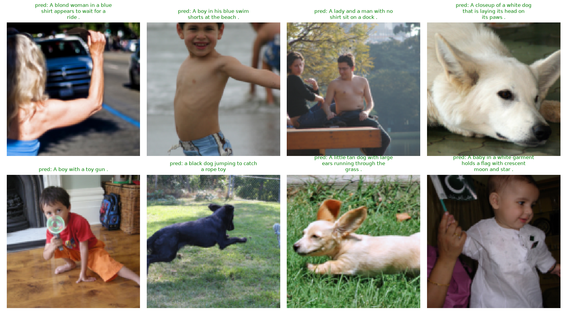
8/8 correct on image→caption. The reverse direction (caption→image, printed to console, not pictured) got 6/8 — the two misses were both photos of young boys in casual outdoor/indoor scenes, a believable confusion given how similar the captions read. Genuinely satisfying to watch a model I built from patch embeddings up get real, checkable answers right.
A hypothesis, tested — and a confound I didn’t catch until the numbers were in. Looking at the
overfitting onset, I noticed something about how the training data was being fed in: the dataset
wrapper picks one of the 5 valid captions per image, at random, each epoch — meaning any single
epoch only trains on 6,000 (image, caption) pairs, even though 30,000 exist. My hypothesis: this
limits how much caption diversity the model sees per epoch, making it easier to memorize
whichever specific phrasing it happened to draw rather than being forced to reconcile several
different valid descriptions of the same image. So I added a flatten_captions option — every
(image, caption) pair becomes its own row, all 5 used every epoch instead of 1 — and reran, same 20
epochs, same everything else.
Naively comparing the two runs epoch-for-epoch, the flattened run looks like a disaster: by epoch 20 it hits 98.8% train accuracy against val accuracy stuck at 15.8%, and val_loss balloons to 5.92 — a far uglier gap than the baseline’s 38.1% / 15.2% / 3.62. My first reaction was that the hypothesis was just wrong. It wasn’t — the comparison was.
Flattening the captions gives each epoch 5x more rows (30,000 vs. 6,000), which means 5x more gradient steps per epoch (468 vs. 93). “20 epochs” stopped meaning the same amount of training the moment I changed how many rows an epoch contained — the flattened run’s 20 epochs are actually ~9,360 total gradient steps against the baseline’s ~1,860. Lining the two runs up by step count instead tells a completely different story:
| ~total steps | baseline (epoch) | val_acc / train_acc / val_loss | flattened (epoch) | val_acc / train_acc / val_loss |
|---|---|---|---|---|
| ~1,400 | 15 (best val) | 15.7% / 32.0% / 3.56 | 3 | 15.4% / 21.1% / 3.47 |
| ~1,860 | 20 (final) | 15.2% / 38.1% / 3.62 | 4 | 15.8% / 28.2% / 3.48 |
At matched step counts, the flattened run reaches equal-or-better validation accuracy with a meaningfully smaller train/val gap and lower val_loss — exactly what the original hypothesis predicted. The hypothesis held up; my experiment design didn’t. I’d fixed epoch count to keep the comparison simple, without registering that an epoch had stopped being a consistent unit of measurement. The honest fix, and the actual next step, is to hold total gradient steps constant across both runs instead of epoch count — a cleaner experiment than the one I ran, not a settled conclusion yet.
What I learned
- The two projection layers (image and text) look identical at a glance but exist for different structural reasons — one is forced by shape-matching to a residual stream, the other is a free choice made specifically so two independently-sized encoders can be compared. Pattern-matching on “it’s a linear layer that changes dimensionality” isn’t enough; the why behind each one is different, and that mattered more than the shape.
- InfoNCE isn’t a new loss — chasing its lineage (NCE → word2vec → CPC → CLIP) made it obvious that contrastive learning has been the same trick, reused, for over a decade. Recognizing “this is just cross-entropy in a specific arrangement” made the whole method feel much smaller and more approachable than the name suggested.
- Building an actual counterexample (the 3×3 “generic caption” matrix) taught me the row/column loss distinction far better than being told “you need both directions” ever could have — I’d recommend constructing a concrete failure case over trusting an explanation, whenever a “why do we need X” question has a numeric answer available.
- A number alone doesn’t tell you if a model is actually aligning modalities or just fitting a loss curve — the 8/8 real prediction grid was more convincing to me than the 15.7% val accuracy number by itself, same lesson as Phase 1’s prediction grid.
- Comparing two training runs by epoch count is only valid if an epoch means the same amount of work in both. The flattened-captions run trained 5x more gradient steps per epoch than the baseline, so the naive epoch-for-epoch comparison made a correct hypothesis look wrong. Re-comparing at matched step counts flipped the conclusion entirely — “total gradient steps,” not “epochs,” is the unit I should have been comparing on from the start.
Code, configs, and full results are in the embodied-gpt repo.