The Sparsity Knob That Did Nothing: Training SAEs and Crosscoders From Scratch

Part of rl-crosscoder — the training companion to the model-diff post, which borrowed the crosscoder trained here.

I turned the sparsity knob up 60×. Nothing happened.

I was training a crosscoder — a sparse autoencoder with a twist — and its whole job is to explain each activation with a handful of features. The knob that’s supposed to control that is the L1 coefficient: crank it up, the model is pushed to use fewer features. I swept it across a 60× range, expecting the active-feature count (L0) to fall toward a few dozen. Instead it sat, stuck, around 1,900 features per token — nowhere near sparse — while a fifth of the dictionary quietly went dead.

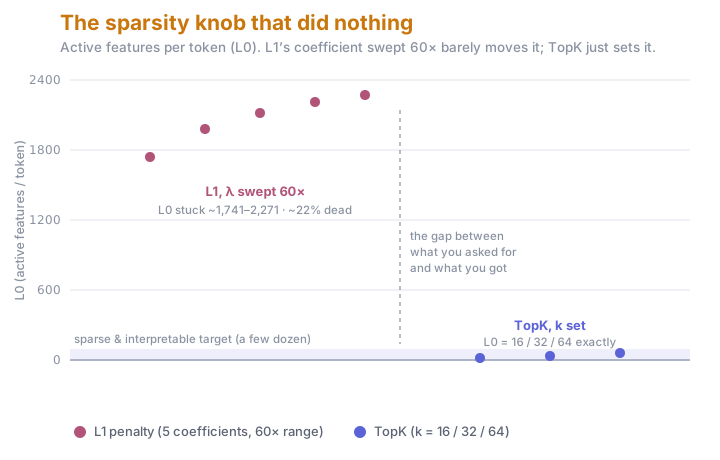
The knob was connected to nothing. And the reason turns out to be the single change that separates a crosscoder from an ordinary SAE — the one change that makes it useful is the same one that silently cuts the wire. This post builds both models from scratch, small enough to hold in your head, and the whole arc is chasing down why that knob is dead and what to use instead. What the trained crosscoder then says about RL is a separate story; here it’s purely how you get one to train.

What we’re building, and why not the obvious thing

The motivating question is model-diffing: take one 1B model before and after an RL step and ask what changed inside. You can’t read the answer off the weights (RL’s weight change is so small it sits at the bf16 rounding floor), and you can’t read it off raw activations either — “these 2,048 numbers shifted a bit” is not something a human can interpret.

So you decompose the activations into something legible. That’s what a sparse autoencoder does, and it’s worth saying exactly what “legible” buys you: an SAE learns an overcomplete dictionary of directions and re-expresses each dense activation as a sparse combination of them — and those directions often turn out to be nameable features (“this fires on Let's think step by step”). The recipe traces to Anthropic’s Towards Monosemanticity (2023).

The obvious plan is then: train one SAE on the before model, one on the after model, compare the two dictionaries. That’s the trap. Two independently trained SAEs give you two dictionaries with no shared index — is feature #4011 in dictionary A the same concept as #206 in dictionary B, or did it split, or vanish? You’re reduced to fuzzy nearest-neighbour matching between two bases, and every claim about “what changed” is downstream of how good that matching was. The confound is baked in on day one.

A crosscoder (ckkissane’s model-diff replication, after Anthropic) walks around that by never building two dictionaries. One shared encoder, one shared feature dictionary — but a separate decoder per model. Each feature exists once, and each model gets its own decoder column for it. Compare the two columns’ norms and you read, per feature, how much each model relies on it — no matching step, ever.

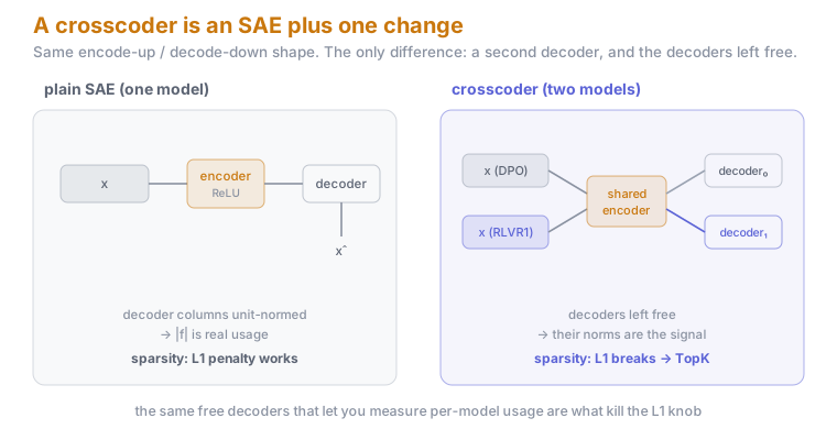
The figure is the whole thesis in one picture: the crosscoder is the SAE with a second decoder head, and with the decoders deliberately left free. Hold onto that word “free” — it’s the villain.

Build the SAE first (and actually train it)

Before writing a line of crosscoder, I trained a plain SAE on a single model’s stream at a single layer. Not because I needed it, but because it exercises the entire data → normalize → train → diagnose pipeline with the simplest possible model on top. If the plumbing is broken, I want to find out with one encoder and one decoder — not while also debugging a second decoder head.

Here’s the whole SAE. It’s two linear layers and a ReLU:

class SAE(nn.Module):
    def __init__(self, d_model, d_hidden):          # 2048 -> 8192 -> 2048
        self.encoder = nn.Linear(d_model, d_hidden)  # project UP
        self.decoder = nn.Linear(d_hidden, d_model)  # project DOWN

    def encode(self, x):
        return F.relu(self.encoder(x - self.decoder.bias))  # pre-center, up, ReLU
    def decode(self, f):
        return self.decoder(f)

    @torch.no_grad()
    def normalize_decoder(self):
        # keep each decoder column unit-norm so |f_j| means "how much feature j is used"
        self.decoder.weight.data = F.normalize(self.decoder.weight.data, dim=0)

The training loop is reconstruction MSE plus an L1 penalty on the features, and — the line that matters most — a normalize_decoder() call after every optimizer step:

x_hat, f = sae(x)
recon = F.mse_loss(x_hat, x)
l1    = f.abs().sum(1).mean()          # plain L1, because the decoder is unit-norm
loss  = recon + cfg.l1_coef * l1
loss.backward(); opt.step()
sae.normalize_decoder()               # <- this is what makes the L1 above meaningful

Why does unit-normalizing the decoder matter? Because L1 penalizes |f_j|, and we need |f_j| to be an honest measure of how much feature j is used. If the decoder column for feature j were free to grow, the model could keep a feature’s contribution to the reconstruction large while shrinking |f_j| to dodge the penalty. Pinning every decoder column to unit norm closes that door: the only way to reduce |f_j| is to genuinely use the feature less. The penalty is meaningful only because the thing it measures is pinned down. File that sentence away.

Trained end-to-end on one layer’s residuals, the SAE came out clean: FVE 0.80, L0 119, 0% dead features. Reconstructs most of the variance, sparse-ish, nothing dark. That “0% dead” was the point of the exercise — it told me the data pipeline, the normalization, and the training loop were all sound, so when the crosscoder later misbehaved I’d know the problem was the crosscoder, not the plumbing. Cheap insurance, and it paid out immediately.

The crosscoder: one shared encoder, two free decoders

Now add the second model. The crosscoder is the SAE with the model axis threaded through — one encoder and one decoder per model, and an encode that sums the models’ contributions into a single shared feature vector:

def encode(self, x):                    # x: (B, n_models, d_model)
    pre = self.b_enc + sum(self.encoders[m](x[:, m] - self.decoders[m].bias)
                           for m in range(self.n_models))
    z = F.relu(pre)                     # ONE shared feature vector explaining both streams
    ...                                 # (sparsify — see below)

def decode(self, f):                    # -> (B, n_models, d_model)
    return torch.stack([self.decoders[m](f) for m in range(self.n_models)], dim=1)

Two design choices carry the whole idea:

• The encoders sum; the decoders don’t. Both streams project up and add before the ReLU, so a single feature vector f has to explain both models. But decoding fans back out through separate per-model decoders. Shared understanding, separate reconstruction.
• The decoders are left free — no normalize_decoder(). This is the deliberate reversal from the SAE, and it’s the entire reason a crosscoder exists: the decoder norm is the measurement. The readout is four lines:

def relative_norms(self):               # (d_hidden,) in [0, 1]
    n = self.decoder_norms()            # ‖dec_m,j‖ per model, per feature
    return n[1] / (n[0] + n[1] + 1e-9)  # ~0 = model-0-only, ~0.5 = shared, ~1 = model-1-only

That vector is the point of the whole apparatus — a per-feature statement of who uses what, sitting in the weights the moment training ends, no matching required. But look what we just gave up. We un-pinned the decoder norm. And the SAE section ended on: the L1 penalty is meaningful only because the thing it measures is pinned down.

The knob is dead, and here’s exactly why

With free decoders, plain L1 on |f_j| no longer means anything (a feature can grow its decoder to stay influential while shrinking |f_j|), so the textbook fix is a decoder-norm-weighted L1: penalize f_j · ‖dec_j‖ instead — the activation scaled by the size of the decoder it feeds. Sounds right. It has a fatal symmetry.

Pick any feature j and any scalar α. Multiply its activation by α and its decoder columns by 1/α:

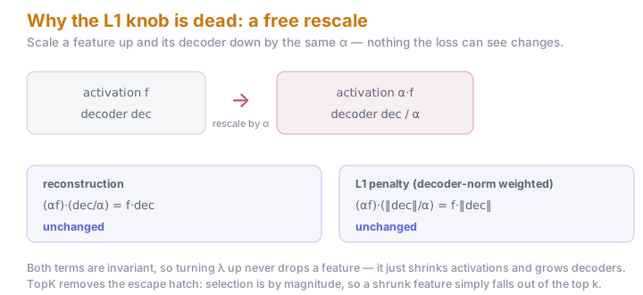
Both the reconstruction and the penalty are invariant — the αs cancel in each. This is a gauge freedom: an entire zero-cost direction the optimizer can slide along. So turning λ up doesn’t push the model to drop features; it just rescales activations down and decoders up to match, leaving L0 exactly where it was. That’s the dead knob from the top of the post, now with a mechanism: a 60× sweep moved L0 by ~23% (from ~1,741 to ~2,271 — the wrong direction, even) while dead features climbed to ~22%. The coefficient was rescaling the model, not sparsifying it.

The fix is to stop encouraging sparsity with a penalty and start enforcing it structurally. TopK (Gao et al. 2024): after the ReLU, keep the k largest features per token and hard-zero the rest.

vals, idx = z.topk(self.k, dim=1)                    # keep the k biggest features/token
return torch.zeros_like(z).scatter_(1, idx, vals)    # everything else -> 0

Two things happen at once. L0 is now exactly k — you don’t tune a coefficient and pray, you set the sparsity directly. And the gauge freedom is gone: selection is by activation magnitude, so a feature that shrinks its own activation to hide from a penalty would simply fall out of the top-k and stop reconstructing. There’s nowhere to hide. The loss drops back to pure reconstruction, no penalty term at all, and the crosscoder trains cleanly:

sparsity	L0 (active/token)	FVE	outcome
L1, coef swept 60×	1,741–2,271 (stuck)	0.97–1.00	dense; ~22% dead; useless split
TopK k=16 / 32 / 64	16 / 32 / 64 (exact)	0.79 / 0.84 / 0.87	sparse, legible

Note the L1 rows have higher FVE — of course they do, ~1,900 features reconstruct almost perfectly. High reconstruction with no sparsity is exactly the failure mode; it’s a reminder that the loss going down is not the metric you care about. The three diagnostics I actually watched every run were FVE per model (is it reconstructing both streams?), L0 (the sparsity you actually got), and dead fraction (a few percent is fine; a fifth is an alarm).

Proof the dictionary learned something real

FVE tells you the crosscoder can rebuild activations; it doesn’t tell you the features mean anything. The honest test is to open the dictionary: take a feature, find the tokens across the whole corpus where it fires hardest, and read them. Here’s a sample from the layer-12 TopK dictionary — the features most selective for reasoning tokens («token» marks the exact firing position):

feature	fires hardest on	reads as
2544	Let«'s» think step by	the step-by-step trigger itself
238 / 7447	«How» many more	the question-word pivot into a problem
3257	If Sally had $20 less, «she would»	a hypothetical / conditional setup
7850	$2 per «jar»	unit-pricing structure in a word problem

These aren’t cherry-picked — they’re the top of the ranked list, each firing almost entirely on reasoning text and near-never on plain prose. A single shared dictionary, trained on both models at once, carved activation space into directions a human can name. The encoder and TopK did their job.

What you have at the end, and what to distrust

You end with one dictionary that reconstructs both models, plus — for free, in the decoder norms — a per-feature relative_norms() readout of how each model uses each feature. That vector is the entire reason to prefer a crosscoder over two SAEs.

Two honest caveats, both about the method rather than any particular finding. First, when I actually read the per-model split out of this run, it was diffuse — the decoder-norm ratio sat near 0.5 for essentially every feature (std ~0.001), so there was no clean set of discrete “RL-only” features to point at. Encouragingly, the L1 and TopK runs collapsed to the same near-0.5 split, which argues it’s a real property of this model pair and not a sparsity artifact — but it means the payoff needed a subtler, correlational analysis, which is its own post. Second, naive crosscoders are known to sometimes invent model-specific features that aren’t real; BatchTopK and latent-scaling crosscoders are the standard hardening, and I left them as the next lever to pull.

But the training lesson generalizes well past this one model, and it’s the thing I’d want you to keep: a regularizer only works if the quantity it penalizes is pinned down. A unit-normed decoder pins |f_j|, so L1 is meaningful in a plain SAE. Free the decoders — the very thing that lets a crosscoder measure per-model usage — and the same penalty becomes a no-op you can sweep 60× with no effect. If you ever adapt an SAE recipe and a sparsity knob feels dead, check whether you removed the normalization that gave it meaning.

Code: sae.py · crosscoder.py · train.py. The trained crosscoder is on the Hub.