Building a World Model From Scratch, Part 1: A Latent Worth Planning In
Part of latent-dynamics, a from-scratch build of a visual world model for CartPole. This is Part 1: turning pixels into a latent. Later parts learn dynamics in that latent, imagine short futures, and plan through them.
I fed my CartPole autoencoder a pole hanging straight down, a cart shoved off the edge, a plain blue square, and a frame of pure noise. None of these is a picture CartPole can ever produce. Here is what a model that has only ever seen CartPole did with them:
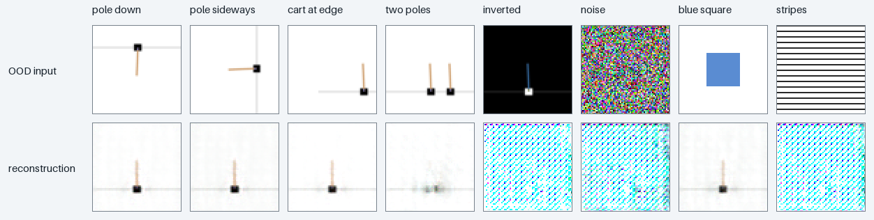
Several came back as a normal, upright cart. The pole pointing down was redrawn pointing up. The blue square was redrawn as a cart. The model has exactly one picture it knows how to paint, and it painted that no matter what I gave it. The ones with inverted colors or pure noise decode to meaningless static instead.
That happens because this model’s entire world is 128 numbers, and those numbers only encode CartPole. Which is exactly what I set out to build. This is Part 1 of a visual world model, and this component’s whole job is to squeeze a 64×64 CartPole frame into a latent short enough that a dynamics model and a planner can run on it. A latent that narrow is the point. It is also the reason the decoder can only draw CartPole, which becomes a real problem for planning later. First, let me build the thing, then come back to why that figure is a warning.
Why compress at all
The goal of this project is a world model: a thing that can look at CartPole, imagine what happens if it pushes left versus right, and pick the action whose imagined future looks best. Model-free RL learns a reflex from state to action. A world model instead learns the environment, then plans inside its own head before touching the real thing.
The loop looks like this:
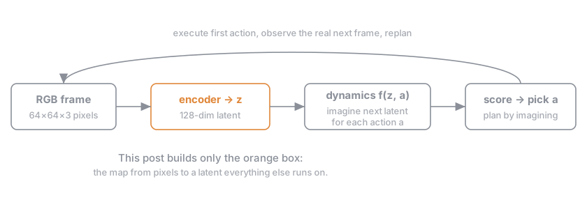
Read left to right. A frame becomes a latent z. A dynamics model f(z, a) predicts the next latent given an action. You roll that forward for a few steps under each candidate action sequence, score the imagined futures, execute the first action of the best one, then look at the real world again and replan.
Every box after the first one operates on z. The dynamics model predicts latents, not pixels. The planner compares latents. So before any of that can exist, I need an encoder that turns a frame into a z compact enough to learn dynamics on and faithful enough that the physics is still in there. That encoder is this post.
Could you skip the latent and predict raw pixels forward in time? People do, and video-prediction world models are a real line of work. But predicting 12,288 pixels per step, most of them white background, spends the entire model on painting walls. A CartPole frame has maybe three degrees of freedom that matter: where the cart is, the pole’s angle, and roughly its angular velocity. Compress to a small vector first and the dynamics model gets to work in a space where almost every dimension could carry signal. That is the bet.
The autoencoder, built by hand
An autoencoder is the simplest way to learn that compression without labels. Two halves. The encoder crushes the image down to a bottleneck vector. The decoder expands the vector back to an image. Train them together to make the output match the input, and the bottleneck is forced to keep whatever the decoder needs. No labels, no privileged state, just pixels in and the same pixels out.
The encoder is three stride-2 convolutions that halve the resolution each time, 64 → 32 → 16 → 8, then a linear layer to the 128-dim latent:
class Autoencoder(nn.Module):
    latent_dim = 128

    def __init__(self):
        super().__init__()
        self.encoder = nn.Sequential(
            nn.Conv2d(3, 32, 4, stride=2, padding=1), nn.ReLU(),    # 64 -> 32
            nn.Conv2d(32, 64, 4, stride=2, padding=1), nn.ReLU(),   # 32 -> 16
            nn.Conv2d(64, 128, 4, stride=2, padding=1), nn.ReLU(),  # 16 -> 8
        )
        self.to_latent = nn.Linear(128 * 8 * 8, self.latent_dim)   # 8192 -> 128
The decoder is the mirror image: a linear layer back to 8×8×128, then three transposed convolutions that double the resolution back up to 64×64×3. The forward pass is just decode(encode(x)), and the loss is pixel MSE against the input. That is the entire model.
One number is worth pausing on. The whole thing is 2.44M parameters, and the two linear layers at the bottleneck (8192 → 128 and back) are 86% of them. The convolutions that actually look at the image are a rounding error, about 165k parameters each way. Almost the entire parameter budget is spent on the single fully-connected squeeze into 128 dimensions and the expansion back out. The part that feels like “the vision” is tiny; the part that feels like plumbing is the model. Worth knowing before I go blaming a blurry pole on the convolutions.
Trained on the 50k frames for 20 epochs of MSE, with the numbers a couple of sections down, here is what it reconstructs on held-out frames it never saw during training:
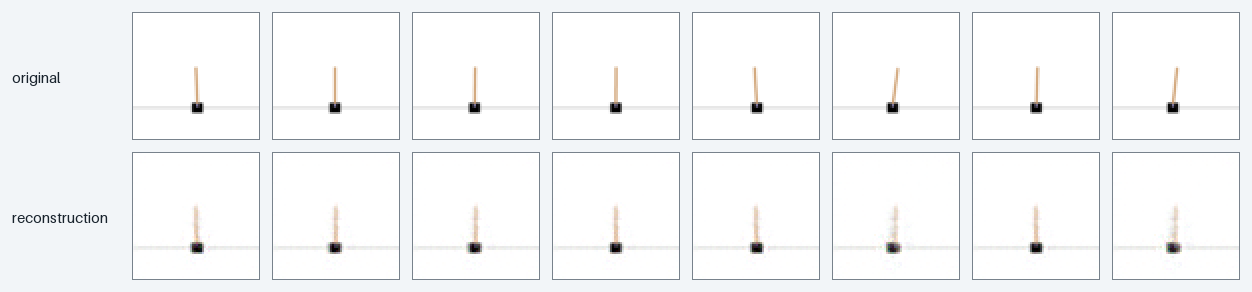
Look at the cart first. The black box is crisp and lands in the right place every time, and the white background is essentially perfect. Now look at the pole. It comes back as a faded, low-contrast bar that thins toward the top, where the original is a solid tan line. The base of the pole is clearly readable; its upper extent is a guess. The model reconstructed the easy, high-contrast cart confidently and got shy exactly on the thin thing that carries the physics. The two clearly tilted poles in this strip, columns six and eight, keep their lean, but they come back noisiest of all: the tilt survives, the crispness does not.
I do not need the picture back. I need the 128 numbers to still know where the cart is and which way the pole is leaning. Everything I build after this runs on those numbers, not on pixels.
The trap: MSE does not care about the pole
Here is the thing that makes this harder than it looks, and it only becomes visible once you know the objective. Look back at a CartPole frame. It is mostly white. The cart is a small black rectangle, the pole is a thin bar a couple of pixels wide, and there is a faint gray track. If I score reconstructions by mean squared error over all 64×64×3 = 12,288 pixels, the background dominates the sum. A model can drive MSE way down by painting a clean white frame with a gray smudge near the middle and never getting the pole angle right.
So the loss I am optimizing and the thing I actually want are not the same thing. MSE rewards getting the wall color right. I want the two pixels that encode the pole’s tilt, because that tilt is the physics. This is the same gap you hit everywhere in this kind of work: the cheap-to-measure proxy and the thing you care about point in almost, but not quite, the same direction, and the model happily walks the gap.
For this milestone I am letting MSE win anyway, because the milestone says to. Blurry is acceptable as long as cart position and pole orientation stay legible. The reconstructions above show exactly that tradeoff: crisp on the high-contrast cart, faded on the thin pole. But I am writing the trap down now because it is the first place I expect the later dynamics model to struggle. If the encoder quietly throws away angular precision to save MSE, no dynamics model downstream can recover it. You cannot plan on information the latent already deleted.
Training, and where the error lives
The dataset is 50,000 pixel transitions collected under a uniform-random policy, seed 42, split 45,000 / 5,000 into train and validation. The split is contiguous, not shuffled: the last 5,000 transitions in collection order become validation, so whole episodes land on one side of the split rather than leaking frame-to-frame neighbors across it. Storage is deliberately dumb, raw uint8 frames on disk, which costs 600 MB for obs alone and buys a format I can memory-map and reason about. Twenty epochs, Adam at 1e-3, batch size 128, MSE loss, on an M4 Pro over MPS.
The numbers, from the actual run:
| metric | value |
|---|---|
| final train MSE (epoch 20) | 0.000475 |
| best validation MSE (epoch 19) | 0.000497 |
| validation PSNR | 33.0 dB |
| train/val gap | negligible |
Two things about that run are worth reporting because they are not the smooth curve you would draw from memory.
First, it was not monotonic. Training MSE started near 0.025, and then at epoch 6 it spiked back up to 0.046, worse than the untrained-ish first epoch, before recovering over the next few epochs. That is Adam at 1e-3 with no learning-rate schedule occasionally stepping off a cliff and climbing back. Nothing to fix at this scale, but the loss did not fall in a clean line, so here is the bump.
Second, most of the gain arrived late. From epoch 7 through 17 the model inched along in the 0.0012 to 0.0018 range, looking basically converged. Then epochs 18, 19, and 20 dropped it hard, validation MSE going 0.00110 → 0.00076 → 0.00050. The model found a better basin in the last three epochs of a twenty-epoch budget. If I had trusted the flat middle and stopped at epoch 15, I would have shipped a visibly worse encoder. Twenty epochs was not overkill here; it was barely enough. The train and validation curves sit right on top of each other the whole way, so there is no overfitting to speak of, which makes sense: 45,000 frames of a three-degree-of-freedom system is a lot of data for a 128-dim bottleneck.
Two more checks on the held-out set, past the single MSE number:
- Where does the error concentrate? I measured reconstruction MSE per image column across 1,000 validation frames. It is exactly where it should be: the central strip where the cart and pole live carries 118× more error than the white margins, peaking at columns 31 and 32, dead center where the pole pivots. The background is reconstructed almost losslessly. The model spends its entire error budget on the moving parts, which is the good outcome. It is also the mechanical reason the aggregate MSE looks so tiny: thousands of trivially-perfect white pixels drag the average down, exactly the dilution the trap section warned about.
- Does the pole angle survive? Partly. Cart position survives cleanly. Pole angle is readable near the base but degraded up the shaft, because the pole is a two-pixel-wide sliver and MSE barely pays for it. So the latent is keeping position well and keeping angle approximately. Whether “approximately” is good enough is not a question I can answer from reconstructions. It is a question for the dynamics model, which will need the encoder to have preserved angular velocity, a quantity that lives in the difference between two of these already-soft poles.
The decoder can only draw CartPole
Now back to the figure that opened this post. Those eight inputs were off-manifold on purpose, each a state CartPole can never render: a pole hanging down below the cart, a pole knocked sideways, the cart shoved to the far edge, two carts at once, a color-inverted frame, pure noise, a blue square, and horizontal stripes. The reconstructions under them split cleanly in two, and both halves say something.
The inputs that still read as a compact shape on a white field get snapped back onto the manifold. The pole hanging down is redrawn pointing up. The sideways pole is stood back upright. The cart shoved to the edge drifts back toward center. Even the blue square, which is not a cart at all, is confidently decoded as a cart with an upright pole. The two-pole frame is the messiest of this group, coming back as a single smeared cart, as if the decoder tried to average two carts into one. The decoder has one thing it knows how to draw, an upright CartPole, and it draws that regardless of what went in. It is not reconstructing these inputs. It is finding the nearest CartPole and rendering that.
The three inputs whose pixel statistics are wrong, the color-inverted frame, the noise, and the stripes, fall off the manifold entirely and decode to a cyan checkerboard artifact. The encoder has no latent code for “mostly black” or “high-frequency noise”, so the decoder renders something structured and meaningless.
For a world model, the first half is the one to worry about. Later I will train a dynamics model that moves around in this latent space, and a planner that searches for latents with good scores. Nothing stops that search from wandering to a latent that no real frame maps to. When it does, the decoder will not error out or look broken. It will hand back a clean, confident, upright CartPole. A planner optimizing against the score of a decoded imagination can exploit exactly this: find an off-manifold latent that decodes to something the score model loves, and chase a future that cannot happen. The milestone notes flag planner exploitation of model error as an interesting failure to preserve rather than patch, and this figure is the pixel-level preview of why it is possible. The map from latents to images is not injective in the direction that matters, and the decoder fails silently.
What this buys, and what is next
Stepping back: this post did the least glamorous piece of a world model, and it is the piece everything else stands on. The encoder is the map from a 12,288-pixel frame to 128 numbers. If those numbers carry the physics, the rest of the project has a place to happen. If they do not, no downstream cleverness gets it back.
The plan from here is the standard world-model recipe, one piece at a time. Freeze this encoder and decoder. Train an action-conditioned dynamics model f(z, a) that takes the current latent plus a left/right action and predicts the next latent, so I can imagine one step forward without rendering a single pixel. Then check the thing that always breaks: one-step predictions can look fine while recursive rollouts drift, because each imagined step feeds the next and small errors compound. I expect that drift, and the plan is to measure how fast it grows before touching the architecture. After that, a score model and a planner that enumerates short action sequences, imagines each, and picks the best.
The open question I am carrying into Part 2 is the one from the trap above. I optimized for pixels and I need physics, and those are not the same objective. Whether that gap matters shows up the moment the dynamics model has to predict a pole angle the encoder was never really paid to preserve.
Code: latent-dynamics. The autoencoder is in models/autoencoder.py, the training loop in scripts/train_autoencoder.py, the reconstruction and OOD grids in scripts/visualize_reconstructions.py and scripts/visualize_ood.py, and the dataset contract in data/. CartPole-v1, 50k random transitions, a single Apple Silicon laptop.