Building a World Model From Scratch, Part 2: A Single Photo Doesn't Know Which Way It's Moving
Part 2 of latent-dynamics. Part 1 is here: it built the encoder that turns a CartPole frame into a 128-dim latent. This part learns dynamics in that latent and plans through them.
I trained a dynamics model on CartPole frames, flipped every LEFT to RIGHT in the validation set, and reran it. The loss barely moved.
The model had learned to predict the next frame while ignoring the action almost entirely. It wasn’t a bug in the network. The problem was sitting in the data: one image, 20ms later, action never mattered enough to matter.
This is the story of chasing that failure through two wrong fixes before finding the real one, then using the working model to control the real environment.
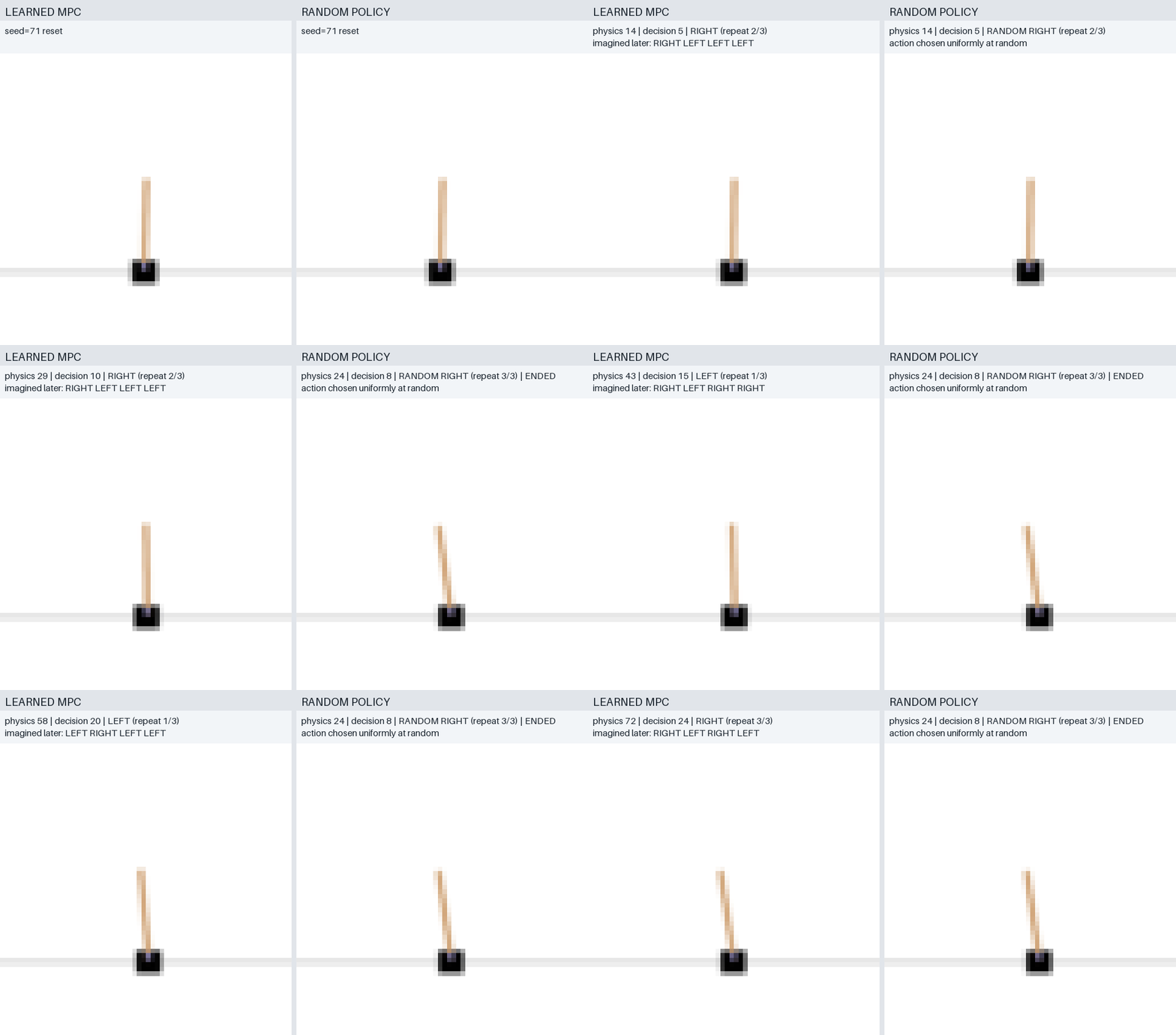
That is the result up front: horizon-5 planning through the fixed dynamics model versus a random policy, same starting seed. Random freezes at physics step 24. The planner keeps going to 72. Getting here took three attempts at the dynamics model.
The setup
The system is a small visual world model for CartPole-v1. Everything that makes a decision, the encoder, the dynamics model, and the planner, sees only rendered 64×64 RGB frames or latents derived from them. CartPole’s simulator state (cart position, cart velocity, pole angle, angular velocity) touches the system in exactly one place, building supervised targets for a score model during training. It never reaches the components that choose actions.
real frames → encoder → imagined futures → score proxy → MPC action
     ↑                                                    ↓
     └──────────── observe, execute, and replan ──────────┘
Notation used throughout:
x_t: the RGB frame at timetz_t = encoder(x_t): its 128-dimensional latenta_t: the action, LEFT (0) or RIGHT (1)f(z_{t-1}, z_t, a_t): the learned next-latent predictor
Attempt one: one frame, one action, ignored
The first dataset stored one CartPole physics step per row: a frame, the action taken, and the frame 20ms later. The dynamics model trained on it and the loss curve looked completely normal. The flip test is what gave it away. Feed the model the correct action, then feed it the opposite action on the same starting latent, and the predicted next latent should move. It barely did.
The cause is in how CartPole itself steps. The action updates the hidden velocities first, and the visible position and angle are updated from the old velocities before that. So one step after LEFT and RIGHT diverge in hidden state, the two resulting images still look almost identical. The model wasn’t broken. It was correctly learning that, for this data, the action barely changes anything a human or a decoder could see.
Attempt two: make the action visible
The fix I tried was to make the effect visible in pixels: repeat the chosen action for three physics steps instead of one, so each stored transition spans 60ms. That worked, as measured by the flip test:
| Validation test | Latent MSE |
|---|---|
| Correct action | 0.00686 |
| Flipped action | 0.00940 |
| Unchanged latent (no-op baseline) | 0.00902 |
Flipping the action now made the one-step prediction 37% worse instead of doing nothing. I took this as the fix and moved on to checking rollouts, where MPC actually has to live.
It wasn’t the fix. Good one-step loss said nothing about what happens when the model’s own output is fed back in as the next input:
| Horizon | Valid sequences | Versus doing nothing |
|---|---|---|
| 1 | 5,000 | 23.9% better |
| 5 | 1,823 | 16.7% worse |
| 10 | 423 | 3.1% worse |
| 20 | 19 | 53.5% worse |
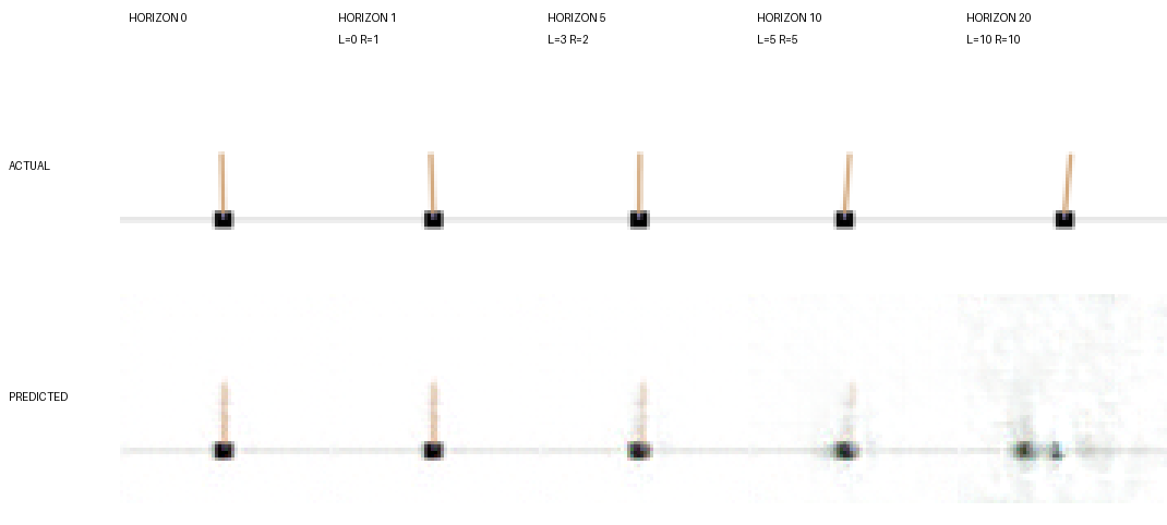
Decoded rollouts stay sharp for a step or two, blur by horizon 5, ghost by horizon 10, and are off the image manifold entirely by horizon 20. The decoder still reconstructs real encoded frames cleanly, so this wasn’t a decoder problem. It was specific to latents the dynamics model invented by recursively feeding on its own predictions, each step’s small error compounding into a state training data never produced.
What was actually missing
Repeat-3 fixed the wrong layer. Making the action’s effect visible in pixels doesn’t help if the input to the model is still a single frame, because a single frame shows where the cart and pole are and says nothing about which way they’re moving. Two physically different states, one drifting left, one drifting right, can produce the same image. No amount of training on that image recovers the missing half of the state.
The fix was to give the dynamics model a second frame, so the difference between two consecutive latents supplies a crude velocity signal:
ẑ_{t+1} = z_t + f(z_t, z_t − z_{t-1}, a_t)
This is closer to a bigram than a sequence model: one frame of history and nothing more. On the same validation data, one-step latent MSE fell from 0.00801 for the single-frame model to 0.00098, an 11.8x drop. This time the rollout numbers moved with it instead of against it:
| Horizon | Better than single-frame |
|---|---|
| 1 | 87.8% |
| 5 | 48.9% |
| 8 | 22.7% |
| 10 | 11.1% |
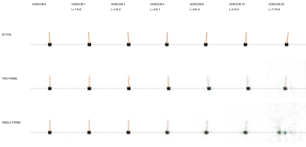
The two-frame model stays coherent out to around horizon 8, which is close to what MPC actually needs. Blur and drift still creep in past that, but no bigger network was involved, just one more frame of context. The lesson from both wrong turns: a one-step loss number tells you almost nothing about whether a model is safe to roll forward, and no amount of capacity fixes a representation that’s missing the relevant state.
Planning through the fixed model
With a dynamics model that finally tracks direction, planning is straightforward. Two actions and horizon 5 means only 2^5 = 32 candidate action sequences, cheap enough to roll all of them forward in one batch. A small score model, trained to rank imagined latents against -(pole_angle² + 0.01 · cart_position²), scores each rollout:
for step in range(horizon):
    next_latent = dynamics(previous, current, sequences[:, step])
    total_scores += score_model(next_latent)
    previous, current = current, next_latent

best = total_scores.argmax()
The controller executes only the first action of the winning sequence, holds it for three real physics steps to match how the training data was collected, then encodes the new real frame and plans again:
decision 4 proposes: RIGHT RIGHT RIGHT RIGHT LEFT
execute now:           RIGHT for physics steps 10, 11, 12
then:                  discard the rest of the guess and replan
Replanning this often means the model only has to rank nearby futures well enough to pick the next action. It doesn’t need to hold a long-horizon plan together, which is good, because horizon 8 is roughly where the dynamics model starts to drift.
Results
Same 100 starting seeds, same repeat-3 execution interval, for both policies:
| Policy | Mean physics steps | Median | Std |
|---|---|---|---|
| Horizon-5 MPC | 31.47 | 29.0 | 14.09 |
| Random | 16.42 | 13.5 | 9.19 |
MPC won 87 of the 100 paired episodes, tied 2, lost 11. Its mean episode is 1.92x the random baseline.
CartPole-v1 caps out at 500 physics steps; this controller averaged 31.47 of them. The best single episode reached 72, ending with the cart nearly centered at x = -0.009 while the pole crossed the failure boundary at -12.75° with angular velocity -1.07 rad/s. The planner learned useful control over a dynamics model that, a few weeks earlier, couldn’t tell LEFT from RIGHT. It did not solve CartPole.
What’s next
The obvious gap is the ending state above: a controller that could see angular velocity directly, rather than inferring it from a frame difference one layer down, would likely have caught that fall earlier. Beyond that, the two-frame dynamics model still drifts past horizon 8, so uncertainty-aware rollouts that discount imagined futures the model is less sure about are a natural next step, along with revisiting whether three physics steps is really the right control interval or just the smallest one that made the original bug visible.
Code: latent-dynamics. Repeat-3 CartPole dataset, same Apple Silicon laptop as Part 1.